


I believe no man ever threw away life, while it was worth keeping. For such is our natural horror of death, that small motives will never be able to reconcile us to it…[DAVID HUME, On Suicide]
According to the World Health Organization, nearly one million people commit suicide each year. This figure translates to a global mortality rate of 16 per 100,000 people, or one suicide every 40 seconds. Among former Soviet republics, the numbers reflect an even grimmer reality: in 2010, the mortality rate from suicide ranged from 27.6 per 100,000 in Kazakhstan to 36.8 per 100,000 in Belarus (WHO 2011). These statistics are naturally troubling; they serve as an indicator of the prevalence of abject despair. Many of these deaths, to be sure, are the outcome of untreated depression and other psychiatric disorders. However, it is not unreasonable to assume that some suicides are “rational,” based on a well-informed cost-benefit analysis. Nor is it unreasonable to assume that these rational analyses take into account economic factors, such as unemployment, inflation, or income. The role that income plays in the suicide decision is of particular interest, as it can help to inform us of how economic development affects lives.
In this paper, I will investigate and evaluate the relationship between income and suicide rates, using data from Russia. I begin by reviewing existing literature, both empirical and theoretical, on the subject. I then model an economic theory of suicide, based on the works of Hamermesh and Soss (1974) and Emile Durkheim (1897). Finally, using regional-level panel data from Russia for the years 1997-2009, I run a fixed-effects generalized least squares regression to empirically estimate this relationship.
Literature Review
The sociological view of suicide is based primarily upon Emile Durkheim’s seminal work, Le Suicide (1897). Durkheim proposed that suicidal behavior stems from one of two sources. The first source relates to the level of social integration within groups and institutions. If an individual lacks strong ties within his social context, or, conversely, over-identifies with his cohort, his or her propensity to commit suicide is higher. The second source pertains to a disparity between means and needs. While Durkheim meant this in a more philosophical sense, he also believed that discrepancies between economic means and needs lead to suicide.
While this theory clearly implies that there is an economic component to suicide decisions, economists generally avoided the topic until the late 20th century (Cameron 2006). Adam Smith (1759) briefly touched upon it in The Theory of Moral Sentiments, arriving at the conclusion that suicide results from psychological derangement rather than logical decision-making. It was not until 1974 that a notable economic theory of suicide, proposed by Hamermesh and Soss, emerged. Their model proposes that a suicide decision is based on utility maximization. Within this framework, a rational agent chooses to commit suicide when his or her total discounted expected lifetime utility falls below some critical threshold. Due to the “materialistic basis of modern society,” this utility is a function of age and income.
Since that time, other noteworthy theories of suicide have emerged within the field of economics. Lester and Yang (1996) proposed a “supply and demand” model of suicide. They suggest that suicide behaves like a “good” traded in a market; the “supply” side of this model can be interpreted as the negative relationship between the costs associated with suicide, such as money, time, and anticipated levels of pain, and the probability of a suicide attempt. The “demand” side can be characterized as the positive relationship between perceived gains from suicide, such as ameliorated suffering, and the propensity to commit suicide.
Shortly after Lester and Yang proposed this theory, Huang (1997) suggested that the suicide decision was analogous to the labor/leisure decision. Just as a worker must decide how many hours to work based on his preferences and budget constraint, a person contemplating suicide must decide how much effort he or she is willing to put into living. The same sort of corner solution that causes a worker to choose unemployment causes an individual in this model to take his own life. The parallels for unearned income that Huang provided for this framework are effortless benefits of living, such as attractiveness or good health. Therefore, he claims, just as an individual who gains a new source of non-labor income is less likely to work, an increase in non-effort benefits increases the likelihood of the suicide. This analogy is theoretically problematic; Whitman (2002) points out the critical fallacy that in order to experience these non-effort benefits, the person must be alive.
Despite the development of these more contemporary models, the majority of economic literature on suicide uses some hybrid of Hamermesh’s and Soss’s model and Durkheim’s theories. The literature yields mixed results as to the precise effect of income on suicide rates. Burr et al. (1997) and Freeman (1998) found that income and suicide have a strong positive relationship. These results support the theory that the extremely poor have resigned themselves to their lots in life, and are therefore less inclined to take their own lives (Durkheim 1897). However, these findings are potentially the result of omitted variable bias; neither paper controls for income inequality, and its effect may have been captured in the income variable (Burr et al. 1997).
These results notwithstanding, most research on the relationship between income and suicide rates indicates that higher suicide rates correspond with lower incomes (Chen et al. 2009). The gender-specific effects of income on suicide are more subject to debate. Looking at data for the United States from 1940-1984, Yang (1992) found that increases in gross national product have a significant detrimental effect on the suicide rates of women, but a beneficial effect on those of men. He provided no explanation, theoretical or econometric, as to why women might be more inclined to commit suicide in the face of economic growth. Chuanc and Huang (1997) found no such detrimental effects of per capita income in their panel analysis of suicide rates in Taiwan. They instead found that while men are more sensitive to macroeconomic variables, suicide rates for both women and men decrease as income increases. Chen et al. (2008) replicated these results in a cross-country analysis of Organization for Economic Co-operation and Development (OECD) countries.
Brainerd (2001) further convolutes the issue in her study of 22 transitioning economies in the 1990s. Like Yang and Chuanc and Huang, she found that male suicide rates strongly respond to macroeconomic indicators such as unemployment and GDP; however, unlike her predecessors, she found that female suicide rates are relatively insensitive to these variables. She proposes that this difference in sensitivity may reflect that “women’s non-market work is valued more highly than men’s in these societies,” providing women with greater protection from macroeconomic turbulence than men. Andres (2005), Walsh and Walsh (2011), and Neumayer (2003) similarly found that only men respond to economic fluctuations in their respective studies of European countries, Ireland, and various other countries.
While there is no strong consensus in prior literature regarding income and suicide rates, a sizeable majority finds a negative relationship between income and suicide among men. The relationship for women is thus far uncertain. Further, there is mixed evidence as to which socio-demographic variables play a role in suicidal behavior.
This paper contributes to existing literature in several ways. First, unlike many of the more recent studies, this study looks at regional level data for just one country, Russia, as opposed to a cross-country analysis. This is a more appropriate approach, as suicides may be reported differently across countries depending on differences in cultural or legal institutions (Hamermesh and Soss 1974). Second, Russia itself is of particular interest; as a G8 nation, it has the resources to a compile a comprehensive statistical database, and yet as a transitioning nation it has experienced rapid economic development, considerable civil unrest, and drastic socio-demographic transformation over the past 20 years. The results may be more informative in assessing what impact economic development may have on suicide rates in developing nations. Further, it has one of the highest suicide rates in the world: 21.4 per 100,000 population in 2011 (WHO 2011). Finally, this paper includes theoretically important variables which prior literature does not, including a measure of urbanization and a variable for war.
Theoretical Framework
This paper models suicide as a rational choice, with both economic and socio-demographic considerations. I base my model on that of Hamermesh and Soss (1974), with some minor adjustments to incorporate Durkheim’s sociological theory of suicide. I begin with the utility function for an average individual of some group with permanent income equal to Y

where m denotes age, C(.) denotes consumption, which is a function of age and income, K(m)represents the cost of maintaining one’s life each year at some minimum subsistence level (assume K’>0), and D(z) is the level of social cohesion, as measured by a vector z of the group’s socio-demographic characteristics. This individual’s lifetime expected utility Z at age amay be expressed as

where r is the rate at which the individual discounts future utility individual discount rate, a* is the maximum life expectancy, and P(m) is the probability of surviving to age m given age a. When total discounted lifelong utility falls below some threshold, the individual commits suicide. This threshold is not necessarily equal to zero; it varies depending on whether living itself contains any utility content (Dixit and Pindyck 1994).
Let bi represent the ith individual’s preference for living, or, alternatively, aversion to dying. biis expressed in comparable units to those in the individual utility function. It may be negative in the case where a suicide attempt has positive utility content (Marcotte 2003). Assume that it is defined at birth. The ith individual will therefore commit suicide at the point where the disutility of continuing to live outweighs the inherent value of life, or
Z(a, Y, D)+bi<0. {3}
The fraction of individuals S in the group born at time (t-a) who commit suicide at age a is therefore[1]:

where f(.) is the density function for bi. Differentiating equation 4 yields

which informs us of the marginal impacts of age, income, and social cohesion on the suicide rate within the cohort. As seen in equation 1, because the cost of living rises with age (K’>0) and remaining permanent income decreases each year, dZ/da<0. The marginal effect of age on expected lifetime utility is likely nonzero, increasing early in life, plateauing in midlife, and increasing again as medical issues associated with age manifest. Overall, d2Z/da2≠0. Conversely, assuming more is preferred to less, expected utility rises with permanent income, so dZ/dY>0. Studies regarding the relationship between happiness and income indicate the marginal utility of additional income decreases as income levels rise, so d2Z/dY2<0 (Scnittker 2008).
dZ/dD depends upon the initial level of social cohesion. Durkheim argues that while suicide often results from a lack of identification with the group, it can also result from over-identification (i.e. suicide bombers or cult members). Despite this, because suicide as a result of extreme social cohesion should occur rarely and in extreme circumstances, I will assume for this model that the relationship between social cohesion and utility is positive; that is, dZ/dD>0. Determining the functional forms of these relationships is a more daunting task, as it requires presumptions as to what makes life worth living (Cameron 2006).
The main predictions of this model are that suicide rates within a group should rise with age and fall with income, life expectancy, and social cohesion. Based on these predictions, I arrive at the guiding equation

where Sit represents the suicide rate, Yit represents per capita income or equivalent measure, LIFEit denotes life expectancy, UNEMPit is unemployment, AGEit is the average age within the cohort, Dit is the vector of socio-demographic which indicate social cohesion, and εit is the stochastic error term. αit captures the incidence of suicide that would exist regardless of these considerations. Literature suggests that vector D consists of religious demographics, migration, divorce rate, inflation, birth rate, female labor force participation, crime rate, income inequality, average age of the population, level of urbanization, labor force demographics, war, and alcohol consumption. Alcohol consumption is particularly important in transitioning economies such as Russia, as it may be used to capture the “stress of transition” (Brainerd 2001, Gruenewald et al. 1995). As in preceding literature, I use the log form of all variables so that the “regression coefficients are comparable” (Yang 1992, Hamermesh and Soss 1974).
The effects of each of these variables should differ between genders if men and women have nonequivalent utility functions. That is,

If equation 6 holds, men and women value economic and socio-demographic variables differently, and will thus make suicide decisions differently. Although I anticipate that men and women will respond differently to the various indicators of social cohesion due to differing societal roles, men and women should respond similarly to changes in income. Specifically, suicide rates for each gender will fall as income rises. Women may even be more vulnerable to economic hardships; with fewer economic opportunities than men, women are often “one divorce away from abject poverty” (Landau 2003).
Data Description
The ideal dataset with which to assess the impact of economic growth on suicide rates would be a balanced panel, containing every relevant variable, for every region in Russia for every year since the fall of the Soviet Union. Unfortunately, various constraints prevent this ideal dataset from being attainable. First, existing literature does not provide an exhaustive list of which variables have meaningful impacts on suicide rates. Suicidal behavior is complex and not perfectly understood, so it is not readily apparent which variables must be included in its study. Second, data for variables which the literature does indicate are important are not always available. For example, Yang (1992) finds that female labor-force participation impacts suicide rates, but this information is not available at the regional level for Russia. Finally, not every region has data for all 20 years since the fall of the Soviet Union. I am therefore left with a somewhat smaller panel than the ideal 20-year, 95-observation panel.
The majority of my data come from the Russian Federal State Statistics Service (Rosstat). Rosstat provides annual national- and regional-level statistics for a number of economic and socio-demographic indicators from 1990-2010. I was able to obtain annual data for the following explanatory variables: gross regional product per capita (GRP) in real terms (rubles), divorces per 1,000 population, convicted crimes per 100,000 population, the percentage of the population which lives in urban areas, unemployment rate, life expectancy disaggregated by gender, net migration per 10,000 population, the number of births per 1,000 population, the number of alcohol-related deaths per 10,000 population, the percentage of the population which is older than working age (59 for men and 54 for women), and the ratio of income Kuznets ratio for the top 10% to the bottom 10%. The number of alcohol-related deaths serves as a proxy for the preferred variable, total alcohol consumption, which was unavailable at the regional level.
I was also able to obtain appropriate data for the dependent variables: suicides per 100,000 population for each gender. There are limitations to what these data can tell us. The figures do not include information on non-fatal suicide attempts, suicides which were never intended to be fatal, or suicides which were miscategorized as another cause of death.
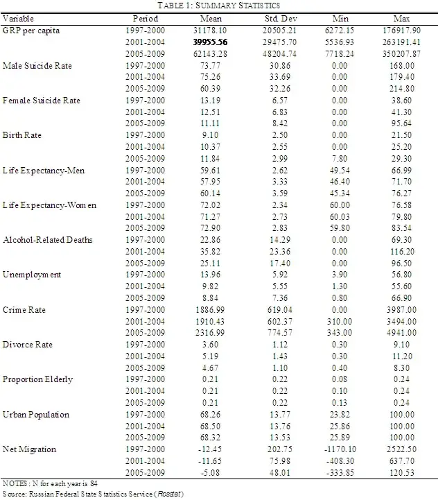
The dummy variable for the Second Chechen War comes from the Office of the United Nations High Commissioner for Human Rights (OHCHR); though there is controversy as to the precise end date of this war, OHCHR, as well as former Russian prime minister Sergei Ivanov, believe that it extended from 1999-2006. Table 1 contains the summary statistics for each variable of the 84 remaining observations in time periods 1997-2000, 2001-2004, and 2005-2009.
- Independent Variables
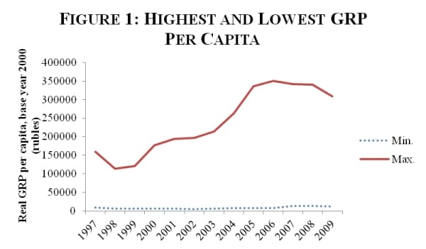
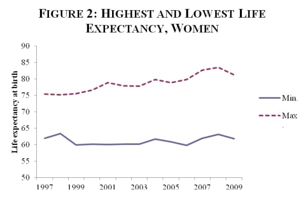
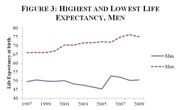
As seen in Table 1, the “average” Russian region experienced rising GRP per capita, birth rate, crime rate, life expectancy, and net migration rate between 1997 and 2009. Meanwhile, unemployment fell, and the prevalence of alcohol-related deaths peaked dramatically in the early 2000s. The urban population and the proportion of population above working age remained relatively unchanged. Most variables have large standard deviations relative to their means, indicating high variability, or, in some cases, extreme outliers. Most remarkably, the GRP per capita for the wealthiest region is 28.2 times larger than that of the poorest between 1997-2000, 47.53 times larger between 2001-2004, and 45.37 times larger between 2005-2009 (see Figure 1). The average GRP per capita for each period was 31,178.10RUB (~US$6,519.33)[2], 39955.56 (~US$8,906.33), and 62,143.28RUB (~$13,943.75). Also striking is the disparity between highest and lowest life expectancies for both men and women. For men, this disparity increased from about 17 years to nearly 31, as seen in Figure 2, and for women, it increased from about 17 years to about 24, as seen in Figure 3.
- Dependent Variables
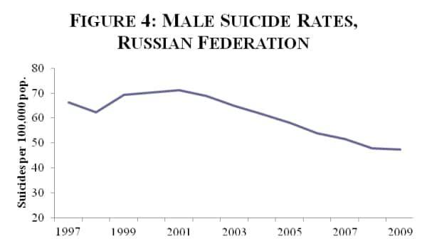
On average, female suicide rates in Russia decreased over time, while male suicide rates rose in the mid 2000s and then fell drastically. Figures 4 and 5 demonstrate these trends. Men have consistently higher suicide rates than women; for example, the average suicide rate for men between 2005-2009 was 60.39 per 100,000 population, nearly six times larger than the average for women, 11.11 per 100,000 population. To put these figures in perspective, the average suicide rate as of 2011 world-wide was 15.3 for men and 4.44 for women (WHO 2011).
Analysis
- Estimation Issues
Suicide may be a response to any number of economic, socio-demographic, or personal characteristics, many of which available data cannot possibly encapsulate. This model therefore lacks a number of important variables. For example, previous literature indicates that female labor force participation, religious demographics, and inflation affect suicide rates (Chuanc and Huang 1997, Andres 2005, Anderson and Kunce 2002), but regional-level data for these variables are unavailable. The exclusion of these variables may bias the magnitude of the estimated coefficients.
Heteroskedasticity and serial correlation often plague panel data. A modified Wald test strongly rejected the null hypothesis of homoskedasticity, despite the logarithmic form of the variables. The Woolridge test for autocorrelation determined that serial correlation is also present in the data. In order to correct for these issues, I used clustered standard errors.
I also needed to determine whether to use fixed or random effects; to do so, I used a Hausman test. The test indicated that fixed effects are preferred—a result confirmed by the Wald test and Breusch and Pagan LM test for random effects. My regressions therefore hold constant time invariant characteristics which differ across regions.
Finally, endogeneity is the most serious estimation issue this model faces. Brainerd (2001) describes the relationship between life expectancy and suicide rates as a “vicious circle”; a lower life expectancy lowers the incentive to invest in living, increasing the probability of suicide, which, in turn, lowers life expectancy. To address this, I attempted to use the instrumental variable “parasite-related deaths per 100,000 population,” but a Hausman test revealed that this was an exceptionally weak instrument. Endogeneity therefore remains unresolved, and will thus bias the estimates.
- Main Results
Table 2 contains the results of the fixed-effects, generalized least squares regression. They indicate that economic and socio-demographic characteristics affect suicide rates differently for men and women. Overall, men seem to be sensitive to fewer variables. At the 5% significance level, higher net migration and incidence of alcohol-related deaths correspond with higher suicide rates, while higher birth rates correspond with lower suicide rates. At the 10% significance level, male suicide rate and GRP per capita are negatively correlated. The coefficient of the variable of interest, GRP, indicates that a 1% rise in GRP corresponds to a 0.116% fall in suicide rates holding all else constant. The suicidal tendencies of men seem most strongly influenced by changes in birth rate; a 10% rise in birth rate corresponds with a 4.07% decrease in suicide rates.
Turning to what Russians refer to as the “more splendid half of humanity,” women, like men, are more likely to commit suicide as the number of alcohol-related deaths increases, and less likely as GRP per capita and birth rate rise. Unlike with men, suicide rates in women increase with divorce rates. Furthermore, women were more likely to commit suicide during the Second Chechen War. Birth rate is also the strongest determinant of female suicide rates, followed by divorce rate: a 10% increase in birth rate corresponds with a 5.2% decrease in suicide rate, while a 10% increase in divorce rate corresponds with a 2.85% increase, ceteris paribus. The model as a whole explains less of the variation in female than in male suicide rates: the R-squared value for male suicides is about .5, whereas it is only .24 for women.
Most of these results are consistent with my expectations. Women likely respond to changes in divorce rate due to their traditional societal roles as wives; a surge in divorce rate results in displacement from these roles. Men suffer from no such role displacement; not only do they more often play other significant societal roles, but in Russia, it may be particularly easy for men to remarry due to the considerably skewed gender ratio created by Russia’s high male mortality rates. Similar dynamics may be driving the difference in sensitivity to war; in times of war, women remain at home while their brothers, husbands, sons, and fathers go off to die. Alone and bereaved, they are more likely to take their own lives, unlike their male counterparts, who are occupied with their patriotic undertakings (or have already died).
Some of the results, on the other hand, are surprising. I expected the proportion of population above working age and crime rate to have positive and significant correlations with suicide rates for both genders. Unable to adapt to an entirely new system so late in life, the elderly in transitioning economies often are most susceptible to economic hardships (Chuanc and Huang 1997). Perhaps it is the case that pensions, in combination with the family-oriented Russian culture, provide older members of society with the support needed to offset these hardships. Alternatively, it may be the case that the elderly, having survived Stalin and the horrors of World War II, are relatively more stoic and less troubled by modern-day woes. As for crime rate, it seems to be an appropriate measure for social disintegration (Brainerd 2001). That is apparently not the case; perhaps higher crime rates are the result of improved law enforcement rather than an actual increase in criminal activity.
Most importantly, the results indicate that, consistent with the theory and findings of Chuanc and Huang (1997) and Chen et al. (2008), increases in gross regional product per capita correspond with lower suicide rates for both men and women. In fact, contrary to the findings of all previous literature, suicides rates of women seem to be slightly more responsive to changes in GRP, falling 1.69% for every 10% increase in GRP, compared to the 1.14% fall in those of men.
- Robustness
- Lagged Independent Variables
It is possible that economic shocks take time to “sink in” before individuals consider them in suicide decisions (Yang 1992). To test this hypothesis, I ran regressions which included the one-year lagged values of unemployment and per capita GRP. Table 3 contains the result of these regressions. The lagged value for per capita GRP has a significant negative relationship with suicide rates for both men and women. The magnitude of the coefficient is in fact greater than that for the current period value (-0.198 for women and -0.193 for men). The lagged value of the unemployment rate has a significant positive relationship with suicide for both sexes, unlike the current period value. Furthermore, life expectancy becomes significant for both genders when holding the lagged economic variables constant.
- Tobit
The disadvantage of linear models is that they often predict impossible y-hat values. In this case, a negative value for suicide rates is theoretically nonsensical. To address this, I ran tobit regressions which censored all negative predicted values of the dependent variable. To impose fixed effects, I included a regional dummy, resulting in a substantial sacrifice in degrees of freedom but an overall more “correct” model. Table 4, column (i) contains the results of these regressions. The coefficients on per capita GRP remain relatively unchanged, but the statistical significance of the results increases appreciably. The results are significant at the 1% level for both men and women
- Remove Outliers
There are a couple of outliers in terms of suicide rates for both sexes within the sample; for men, these are Nenetskii Okrug and Respublica Altai, and for women, Vologodskaya Oblast andKoryakskii Okrug. In order to ascertain whether these outliers biased the estimated coefficients, I ran regressions with the outliers removed. Table 4, column (ii) contains the results for these regressions. The resulting changes in the estimates are small, but nonzero. The coefficient on per capita GRP decreases somewhat for women, and falls in statistical significance to the 10% level, while the same coefficient for men remains the same in terms of magnitude, but increases in statistical significance to the 5% level. The R-squared value remains the same for men, but increases from 0.24 to 0.26 for women.
- Alternate Specification of the Explanatory Variable–GRP growth
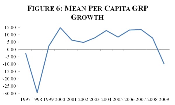
It is of interest not only to assess the impact of income on suicidal behavior, but also the impact of the growth of income. Table 5 contains summary statistics for per capita GRP growth by year. In the late 1990s, GRP actually shrunk for the average Russian region. The majority of the 2000s, however, was characterized by significant growth, with mean annual growth rates ranging from 4.83% to 13.55%.
Table 6, column (i) contains the results of regressions run with GRP growth, in levels, as the independent variable. As expected, the sign is negative, but the results are statistically significant for neither men nor women. A simple correlation test indicated that GRP growth and levels are not strongly collinear (β=0.116), so I ran additional regressions holding both constant. Table 6, column (ii) contains the results of these regressions. In this model, the GRP per capita growth rate is significantly negatively correlated with male suicide rate, with the suicide rate falling 0.1% for every 1 percentage point increase in growth. There is no significant correlation between female suicide rates and growth. Per capita GRP levels, however, are still significantly and negatively correlated with suicide rates for both genders.
Conclusion
This paper examines the relationship between income and suicide rates, using regional-level data from Russia for the years 1997-2009. The evidence presented indicates that there is a statistically significant, inverse relationship between income level and suicide rate. These results apply to both genders and are robust across several different estimation techniques. Unfortunately, due to bias caused by omitted variables and a degree of endogeneity, no definitive conclusions can be drawn from this evidence. Despite these limitations, this paper contributes to the growing consensus that there is an economic component to the decision to take one’s own life. With this evidence in mind, we can assert with more confidence that economic development has a positive impact on people’s lives. Further, policymakers are more equipped to ameliorate suffering and prevent such tragic losses of life.
Works Cited
Andres, A.R. 2005. “Income inequality, unemployment, and suicide: a panel data analysis of 15 European countries.” Applied Economics. Vol. 37, pp. 439-45.
Brainerd, E. 2001. “Economic Reform and Mortality in the former Soviet Union: A study of the suicide epidemic of the 1990’s.” European Economic Review. Vol.45, pp. 1007-1019.
Burr, J.A., C.G. Ellison, and P.L. McCall. 1997. “Religious Homogeneity and Metropolitan Suicide Rates.” Social Forces. Vol. 76 No.1, pp. 273-299.
Cameron, Samuel. 2006. “Economics of Suicide.” Economics uncut: a complete guide to life, death, and misadventure. Northampton.
Chen, J., Y.J. Choi, and Y. Sawada. 2008. “Suicide and Life Insurance.” Center for International Research on the Japanese Economy Discussion Papers. University of Tokyo.
Chen, J., Y.J. Choi, K. Mori, Y. Sawada, and S. Sugano. 2009. “ Socio-economic Studies on Suicide: A Survey.” Center for International Research on the Japanese Economy Discussion Papers. University of Tokyo.
Chuanc, H. and W. Huang. 1997. “Economic and social correlates of regional suicide rates: A pooled cross-section and time-series analysis.” Journal of Socio-Economics. Vol. 26 No.3, pp. 277-289.
Dixit, A. and R. Pindyck. 1994. “Investment Under Uncertainty.” Princeton University Press, Princeton, NJ.
Durkheim, E. “Le suicide.” 1958. Trans. J. Spaulding and G. Simpson. Free Press, New York.
Federalnaya Slujba Gosudarstvenoi Statistici (Rosstat). Regional Block Database. No longer available online as of 2025
Freeman, D.G. 1998.“Determinants of Youth Suicide: The Easterlin-Holinger Cohort Hypothesis Re-examined.” American Journal of Economics and Sociology. Vol. 57, pp. 183-200.
Hamermesh, D. 1985. “Expectations, life expectancy, and economic behavior.” Quarterly Journal of Economics, Vol. 100, 389-408.
Hamermesh, D., Soss, N. 1974. “An economic theory of suicide.” Journal of Political Economy, Vol. 82, pp. 83-98.
Huang, W. 1997. “A ‘Life Force’ Participation Perspective of Suicide.” In D. Lester, & B. Yang, The Economy of Suicide: Economic Perspectives on Suicide (pp. 81-89). Commack, NY: Nova Science Publishers.
Hume, D. 1783. “On Suicide.” Essays on Suicide and Immortality of the Soul.
Kunce, M. and A.L. Anderson. 2002. “The impact of socioeconomic factors on state suiciderates: a methodological note.” Urban Studies. Vol. 39, pp. 155-162.
Landau, C. and M.C. Cyr. 2003. The New Truth About Menopause: Straight Talk About Treatments and Choices from Two Leading Women Doctors. New York.
Lester, D. and B. Yang. 1996. “Conceptualizing suicide in economic models.” 3 AppliedEconomics Letters, pp. 139-143.
Marcotte, D.E. 2003. “The Economics of Suicide, Revisited.” Southern Economic Journal, Vol.69 No.3, pp. 628-643.
Neumayer, E. 2003. “Are Socioeconomic Factors Valid Determinants of Suicide? Controlling for National Cultures of Suicide with Fixed-Effects Estimation.” Cross-Cultural Research, Vol. 37, No.3, pp. 307-329.
Office of the United Nations High Commissioner for Human Rights (OHCHR). 2006. “Statement by the High Commissioner for Human Rights on her visit to Russia.”
Gruenewald, P.J., W.R. Ponicki, and P.R. Mitchell. 1995. “Suicide rates and alcohol consumption in the United States, 1970-89.” Addiction. Vol.90, No.8, pp. 1063-1075
Schnittker, J. 2008. “Diagnosing our national disease: Trends in income and happiness, 1973 to 2004.” Social Psychology Quarterly, Vol.71, No.3, p. 257.
Smith, A. 1759. The Theory of Moral Sentiments. London.
Walsh, B., and D. Walsh. 2011. “Suicide in Ireland: The Influence of Alcohol and Unemployment.” The Economic and Social Review, Vol. 42, No.1, pp. 27-47.
Whitman, D.G. 2002. “A Search Theory of Suicide.” NBER Working Paper Series.
World Health Organization (WHO). 2011. “Suicide Rates per 100,000 by country, year, and sex.” Available online. Web Access: Dec. 6, 2011.
WHO. 2011. “Mental Health: Suicide Prevention and Special Programs.”
Yang, B. 1992. “The Economy and Suicide: A Time-Series Study of the United States.” American Journal of Economics and Sociology, Vol. 51, No. 1, pp. 87-99.
Appendix

| TABLE 2: MAIN REGRESSION RESULTS | ||
| Independent Variables | Female | Male |
| Gross Regional Product Per Capita | -0.169** | -0.114* |
| (-2.27) | (-1.99) | |
| Second Chechen War | -0.067** | 0.02 |
| (-2.02) | (-0.73) | |
| Proportion of Elderly | 0.042 | 0.105 |
| (-0.11) | (-0.38) | |
| Birth Rate | -0.520*** | -0.407*** |
| (-3.95) | (-3.94) | |
| Kuznet’s Ratio (10/10) | -0.086 | -0.113 |
| (-0.82) | (-1.46) | |
| Unemployment Rate | 0.058 | 0.052 |
| (-1.3) | (-1.47) | |
| Crime Rate | 0.025 | -0.013 |
| (-0.4) | (-0.29) | |
| Net Migration | 0.001 | 0.017** |
| (-0.14) | (-2.29) | |
| Alcohol-Related Deaths | 0.131*** | 0.129*** |
| (-3.15) | (-3.25) | |
| Divorce Rate | 0.256** | 0.054 |
| (-2.12) | -0.53 | |
| Proportion of Urban Population | 0.258 | -0.597 |
| (-0.34) | (-0.9) | |
| Life Expectancy | -1.614 | -1.198 |
| (-1.48) | (-1.84) | |
| Constant | 10.263 | 13.542*** |
| (-1.64) | (-3.39) | |
| Observations | 1084 | 1085 |
| Number of Regions | 84 | 85 |
| R-squared | 0.24 | 0.5 |
| Robust t statistics in parentheses *significant at 10% ** significant at 5% *** significant at 1% |
||
| TABLE 3: LAGGED VARIABLES REGRESSION RESULTS | ||||
| Female | Male | |||
| Independent Variables | Current Period | Lagged | Current Period | Lagged |
| Gross Regional Product Per Capita | -0.198** | -0.193*** | ||
| (2.04) | (3.49) | |||
| Second Chechen War | -0.099*** | 0.007 | ||
| (3.73) | (-0.29) | |||
| Proportion of Elderly | 0.005 | 0.176 | ||
| (-0.01) | (-0.69) | |||
| Birth Rate | -0.213 | 0.01 | ||
| (-1.19) | (-0.08) | |||
| Kuznet’s Ratio (10/10) | -0.097 | -0.104 | ||
| (-0.82) | (-1.31) | |||
| Unemployment Rate | 0.125** | 0.131*** | ||
| (2.27) | (2.86) | |||
| Crime Rate | 0.008 | -0.015 | ||
| (-0.14) | (-0.35) | |||
| Net Migration | -0.004 | 0.013* | ||
| (-0.5) | (-1.88) | |||
| Alcohol-Related Deaths | 0.115*** | 0.12*** | ||
| (3.00) | (3.29) | |||
| Divorce Rate | 0.149 | -0.02 | ||
| (-1.19) | (-0.23) | |||
| Proportion of Urban Population | 0.446 | -0.608 | ||
| (-0.63) | (-1.02) | |||
| Life Expectancy | -1.835** | -1.149** | ||
| (2.06) | (2.10) | |||
| Constant | 10.226 | 13.376** | ||
| (-1.85) | (3.90) | |||
| Observations | 1003 | 1004 | ||
| Number of Regions | 84 | 85 | ||
| R-squared | 0.25 | 0.56 | ||
| Robust t statistics in parentheses *significant at 1% ** significant at 5% *** significant at 1% |
||||
| TABLE 4: FURTHER ROBUSTNESS RESULTS | ||||
| (i) | (ii) | |||
| Independent variables | Female | Male | Female | Male |
| GRP Per Capita | -0.162*** | -0.114*** | -0.114* | -0.117** |
| (-3.56) | (-3.59) | (-1.69) | (-2.02) | |
| Second Chechen War | -0.070*** | 0.02 | -0.072** | 0.023 |
| (-3.36) | (-1.27) | (-2.12) | (-0.8) | |
| Proportion of Elderly | -0.01 | 0.105 | 0.195 | 0.111 |
| (-0.08) | (-1.17) | -0.47 | (-0.4) | |
| Birth Rate | -0.488*** | -0.407*** | -0.606*** | -0.415*** |
| (-4.26) | (-5.03) | (-4.61) | (-3.96) | |
| Kuznet’s Ratio (10/10) | -0.086 | -0.113*** | -0.108 | -0.1 |
| (-1.4) | (-2.59) | (-0.99) | (-1.28) | |
| Unemployment Rate | 0.055* | 0.052** | 0.05 | 0.052 |
| (-1.71) | (-2.29) | (-1.12) | (-1.44) | |
| Crime Rate | 0.018 | -0.013 | 0.039 | -0.015 |
| (-0.43) | -0.44 | (-0.62) | (-0.33) | |
| Net Migration | 0.002 | 0.017*** | 0.007 | 0.017** |
| (-0.24) | (-3.39) | (-0.95) | (-2.32) | |
| Alcohol-Related Deaths | 0.119*** | 0.129*** | 0.134*** | 0.128*** |
| (-5.32) | (-7.95) | (-3.17) | (-3.22) | |
| Divorce Rate | 0.231*** | 0.054 | 0.221* | 0.048 |
| (-2.65) | (-0.87) | (-1.84) | (-0.47) | |
| Proportion of Urban Pop. | 0.157 | -0.597** | 0.599 | -0.652 |
| (-0.38) | (-2.05) | (-0.78) | (-0.95) | |
| Life Expectancy | -1.797** | -1.198*** | -2.101* | -1.175* |
| (-2.44) | (-3.92) | (-1.99) | (-1.79) | |
| Constant | 11.710*** | 13.507*** | 10.776* | 13.723*** |
| (-3.42) | (-7.92) | (-1.74) | (-3.34) | |
| Observations | 1084 | 1085 | 1058 | 1072 |
| Number of Regions | 84 | 85 | 82 | 82 |
| R-squared | – | – | 0.26 | 0.5 |
| Robust t statistics in parentheses *significant at 10% ** significant at 5% *** significant at 1% |
||||
| Column (i) contains results from the tobit regression; Column (ii) contains results in which outliers in suicide rate removed | ||||
| TABLE 5: SUMMARY STATISTICS: GRP GROWTH | ||||
| Year | Mean | Std. Dev | Min. | Max |
| 1997 | -2.68 | 8.17 | -23.04 | 21.42 |
| 1998 | -29.40 | 9.27 | -50.04 | 0.21 |
| 1999 | 2.43 | 10.61 | -22.43 | 29.92 |
| 2000 | 14.86 | 11.47 | -4.26 | 83.69 |
| 2001 | 6.42 | 9.48 | -23.47 | 43.73 |
| 2002 | 4.83 | 7.61 | -18.76 | 26.38 |
| 2003 | 8.09 | 5.81 | -21.70 | 20.55 |
| 2004 | 13.04 | 8.97 | -17.24 | 41.58 |
| 2005 | 8.51 | 7.02 | -10.35 | 25.75 |
| 2006 | 13.33 | 5.45 | -4.86 | 26.10 |
| 2007 | 13.55 | 7.86 | -2.34 | 51.44 |
| 2008 | 7.94 | 6.55 | -23.04 | 26.43 |
| 2009 | -9.72 | 10.33 | -42.70 | 30.81 |
| TABLE 6: REGRESSION RESULTS WITH GRP GROWTH | ||||
| (i) | (ii) | |||
| Indpendent Variables | Female | Male | Female | Male |
| GRP Growth | 0 | 0 | -0.001 | -0.001* |
| (-0.1) | (-0.61) | (-1.17) | (-1.89) | |
| GRP Per Capita | – | – | -0.177** | -0.173*** |
| – | – | (-2.56) | (-2.88) | |
| Second Chechen War | -0.054* | 0.037 | -0.045 | 0.045* |
| (-1.86) | (-1.54) | (-1.52) | (-1.83) | |
| Proportion of Elderly | 0.09 | 0.09 | 0.092 | 0.088 |
| (-0.25) | (-0.31) | (-0.25) | (-0.29) | |
| Birth Rate | -0.593*** | -0.483*** | -0.455*** | -0.339*** |
| (-4.45) | (-3.78) | (-3.43) | (-2.9) | |
| Kuznet’s Ratio (10/10) | -0.173 | -0.156** | -0.11 | -0.093 |
| (-1.58) | (-2.16) | (-1.04) | (-1.19) | |
| Unemployment Rate | 0.098** | 0.090*** | 0.056 | 0.049 |
| (-2.46) | (-2.81) | (-1.32) | (-1.38) | |
| Crime Rate | 0.005 | -0.027 | 0.036 | 0.006 |
| (-0.08) | (-0.59) | (-0.54) | (-0.13) | |
| Net Migration | 0.008 | 0.017** | 0.006 | 0.016** |
| (-0.95) | (-2.34) | (-0.77) | (-2.13) | |
| Alcohol-Related Deaths | 0.105** | 0.113** | 0.110** | 0.117*** |
| (-2.25) | (-2.57) | (-2.42) | (-2.66) | |
| Divorce Rate | 0.178 | 0.015 | 0.258** | 0.097 |
| (-1.6) | (-0.16) | (-2.11) | (-0.95) | |
| Proportion of Urban Pop. | 0.301 | -0.583 | 0.232 | -0.636 |
| (-0.39) | (-0.84) | (-0.33) | (-1.01) | |
| Life Expectancy | -2.306** | -1.394** | -1.548 | -1.101* |
| (-2.25) | (-2.06) | (-1.48) | (-1.67) | |
| Constant | 11.996** | 13.470*** | 10.130* | 13.496*** |
| (-2.18) | (-3.58) | (-1.74) | (-3.66) | |
| Observations | 1000 | 1001 | 1000 | 1001 |
| Number of Regions | 84 | 85 | 84 | 85 |
| R-squared | 0.22 | 0.45 | 0.23 | 0.46 |
| Robust t statistics in parentheses * significant at 10% ** significant at 5% *** significant at 1% |
||||
| Column (i) contains results with GRP growth; Column (ii) contains results with both GRP and GRP growth held constant | ||||
